Raster Analysis & Geostatistics using Kriging

---

2.1. Semivariogram analysis

Semivariograms describe how data are related with distance by plotting the semivariance against the separation distance, known as the experimental or empirical semivariogram. The semivariance is defined as half the average squared difference between points separated by some distance h. As the separation distance h between samples increase, we would expect the semivariance to also increase (again, because near samples are more similar than distant samples).

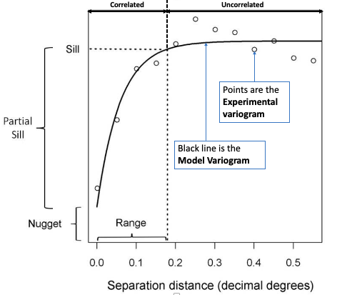
In the generic semivariogram shown above, there are three important parameters:

1. Sill: The maximum semivariance value observed, and it indicates the threshold for values beyond (i.e., flatline) which there is no spatial autocorrelation. NOTE: the Partial Sill is a value calculated by taking the difference between the Sill and Nugget (i.e., Partial Sill = Sill - Nugget)
2. Range: The maximum separation distance h at which we will expect to find evidence of spatial autocorrelation. A separation distance beyond the range samples are no longer correlated.
3. Nugget: This describes the variance of the measurement error combined with spatially uncorrelated variations at distances shorter than the sample spacing, namely noise in the data. The larger the nugget relative to the sill, the less spatial dependence there is in the data and less useful Kriging will be.

IMPORTANT NOTES: Two important assumptions of a basic semivariogram are that the spatial process under investigation are: i.) stationary, i.e., the spatial autocorrelation between the measurements of same variables in a given area is the same for all locations; and ii.) isotropic, spatial autocorrelation is the same in every direction. If the autocorrelation differs by direction, it is termed as anisotropic.

To be used in Kriging, a semivariogram plot (akin to the above image) must be generated to estimate the 3 parameters (i.e., sill, nugget & range) from the points termed experimental or empirical semivariogram. These are used as initial values to fit a modelled or theoretical semivariogram which can be in one of three major forms: 1. Gaussian Model (Left) 2. Spherical Model (Center) 3. Exponential Model (Right)

Once the modelled semivariogram has been defined, it can be used in Kriging.

2.2. Plotting the Empirical Semivariogram

Use the function variogram() to create the object for plotting the empirical variogram

# coerce datafile_sf_prj to be a 'sp' spatial dataframe object as it variogram does not use 'sf' objects
# ignore warning message
datafile_sp_prj <- as(datafile_sf_prj, "Spatial")
# use variogram() function to compute the semivariance with a null model Mean_SO2 as outcome
SO2_emp.variogram <- variogram(Mean_SO2~1, datafile_sp_prj)
# Compute the object to reveal a table
SO2_emp.variogram

##      np       dist    gamma dir.hor dir.ver   id
## 1  1600   80215.64 16.67617       0       0 var1
## 2  2787  243459.82 40.64445       0       0 var1
## 3  4323  399559.96 34.30631       0       0 var1
## 4  5058  554337.13 44.93295       0       0 var1
## 5  5408  710314.24 67.66873       0       0 var1
## 6  5749  867144.10 58.51999       0       0 var1
## 7  6020 1025117.47 72.54208       0       0 var1
## 8  5922 1183536.29 81.79818       0       0 var1
## 9  5204 1340649.65 59.92406       0       0 var1
## 10 5516 1499090.63 39.48967       0       0 var1
## 11 5548 1655939.11 39.47046       0       0 var1
## 12 5368 1811663.84 39.18724       0       0 var1
## 13 4568 1968825.44 37.81360       0       0 var1
## 14 4151 2126333.33 58.96861       0       0 var1
## 15 3718 2284808.08 44.72158       0       0 var1

IMPORTANT NOTES: np in the output is the number of paired considered within the separation distance dist; gamma is the averaged semivariance for the number of paired points within the separation distance dist.

Let us plot these values to see the empirical semivariogram

plot(SO2_emp.variogram)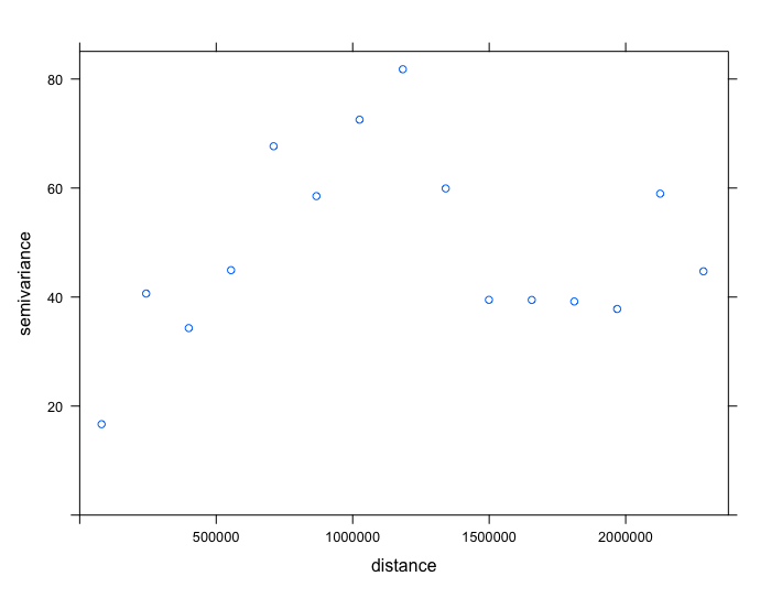

From the output (i.e., plot and table), we should note the approximate values for the partial sill, nugget and range. 1. The nugget is roughly 17 (i.e. base on starting gamma value from the table). 2. The range is roughly 1180000 meters (i.e. base on peak value for gamma and it’s corresponding dist). 3. The partial sill is 65. This is derived from the peak value for gamma subtracted by the nugget (82 - 17 = 65).

These initial values give us an idea of what to expect when we proceed to fit a theoretical semivariogram using the fit.variogram(). It will help us to generate the fitted models.

2.3. Plotting the Theoretical Semivariogram

We are going to fit a model to the empirical semivariogram in order to determine the appropriate function for Kriging (i.e., spherical (Sph), exponential (Exp) or gaussian (Gau)).

We will start fitting the various models:

# Fit exponential
exp_SO2_emp.variogram <- fit.variogram(SO2_emp.variogram, model = vgm(65, "Exp", 1180000, 17))
exp_SO2_emp.variogram
plot(SO2_emp.variogram, exp_SO2_emp.variogram, main  = "Exponential model (Nug: 3.6, PSill: 55.9, Range: 296255m)")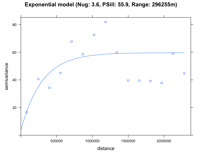

# Fit Spherical
sph_SO2_emp.variogram <- fit.variogram(SO2_emp.variogram, model = vgm(65, "Sph", 1180000, 17))
sph_SO2_emp.variogram
plot(SO2_emp.variogram, sph_SO2_emp.variogram, main  = "Spherical model (Nug: 10.5, PSill: 49.6, Range: 857452m)")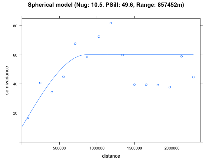

# Fit gaussian
gau_SO2_emp.variogram <- fit.variogram(SO2_emp.variogram, model = vgm(65, "Gau", 1180000, 17))
gau_SO2_emp.variogram
plot(SO2_emp.variogram, gau_SO2_emp.variogram, main  = "Gaussian model (Nug: 12.8, PSill: 39.1, Range: 244807m)")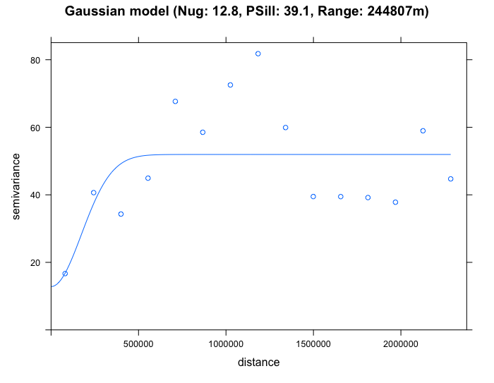

By eyeballing the images - it difficult to discern whether the exponential or spherical model provides a better fit to the empirical semivariogram. We can use the fit.variogram() function to determine which is the best model amongst them.

# select the best model
best_SO2_emp.variogram <- fit.variogram(SO2_emp.variogram, model = vgm(c("Exp", "Gau", "Sph")))
best_SO2_emp.variogram

##   model     psill    range
## 1   Nug  3.628312      0.0
## 2   Exp 55.971076 296255.7

From the output (see column which says model and row 2 it highlights "Exp"), it shows that the exponential model is the best fit with a nugget = 3.6, Partial Sill = 55.9 and Range = 296255m. We therefore select the exponential model in our Kriging to make the spatial prediction for \(SO_{2}\). Lets proceed to Krige.

IMPORTANT NOTES: The interpretation is as follows: the nugget in the exponential model is smaller than the other proposed models. It is small which is also an indication of evidence of larger spatial dependence in the concentrations for \(SO_{2}\) across sampling sites in USA; A separation distance with values beyond 296255m (where it curve starts to plateau) and beyond the semivariance’s threshold where it flat lines (sill of 59.5 (i.e., 55.9 + 3.6)) - there should expect that the spatial autocorrelation in the observed levels of \(SO_{2}\) are not present anymore.

---